Sentiment Analysis of S&P 500 Company Annual Reports
Note:
This article provides a high-level explanation of the underlying analysis, along with some code excerpts and visualizations.
For a comprehensive view of the entire analysis, I encourage you to explore the full Jupyter Notebook, accessible for download on my Kaggle account through the following link.
Tools & Packages used
Python: NumPy, Pandas, NLTK, sci-kitlearn, Matplotlib
SQL
Power BI
Introduction
Motivation
Annual reports (10-Ks) filed by large corporations contain a wide array of financially relevant information. Traditionally, however, analyses of these filings exclusively rely on quantitative measures contained within them. This mean, such analyses are often missing out on extensive narrative data present in these filings. Seeing the potential information gain, an analysis that incorporates textual data should, in theory, be preferred to one that completely omits this kind of information.
Objective
For this reason, this data analysis project sets out to analyze the sentiment expressed in corporate filings (10-Ks). The analysis focuses on filings of S&P 500 companies from 2002 through 2021.
The goal is to identify trends and patterns of corporate sentiment overall and over time. Additionally, the measured sentiment will be linked to subsequent stock returns.
Basic Methodology
Dictionary-Based Sentiment Analysis
Extracting this kind of data, however, is no straight-forward task as textual data is highly unstructured. In finance literature two broad categories for extracting sentiment have been established.
Dictionary-based Approaches
vs.
Machine-Learning-based (ML) Approaches
As the dictionary-based approaches are much more common in the finance academic literature (El Haj et al., 2019, p. 273), the analysis it hand also uses a dictionary to establish the sentiment of company filings. In this context a dictionary simply refers to predefined lists of words. Each of these words is then prelabeled or categorized in accordance with its associated theme, connotation, or sentiment. Typical categories include ‘positive’, ‘negative’, ‘neutral’, ‘uncertain’, etc.
The specific dictionary used for the purposes of this project was introduced by Loughran and McDonald (2011) specifically for the purpose of assessing the sentiment of 10-K filings. It is also by far the most commonly applied dictionary in finance literature.
Accordingly, the analysis follows the procedure suggested by Loughran and McDonald (2011). This involves using the negative word list from their dictionary to calculate a negative sentiment score for each filing. The word list contains 1,993 negative words.
Examples of negatively labeled words from the used word list:
abandon
careless
claim
destabilized
Sentiment Scores - Weighting Shemes
Fundamentally, the sentiment score is derived by tallying the occurrences of any of these pre-labeled negative words within a document. Subsequently, a weighting scheme is applied to determine the final sentiment score for a given filing.
Note: Given the exclusive use of negative words, the computed sentiment score gauges the degree of negativity. In other words, a higher score corresponds to a more negative sentiment expressed in a filing.
In line with Loughran and McDonald (2011) two different weighting schemes are applied resulting in two different sentiment scores for each filing:
(1) Proportional Weighting
Proportional weighting implies adding up the occurrences of all negatively labeled words within a document and weighting this absolute frequency by the total number of words in the document. The proportionally-weighted sentiment score, hence, is simply the relative frequency of the words in the negative word list. Hereby, every word count receives the same weight.
(2) TF-IDF Weighting
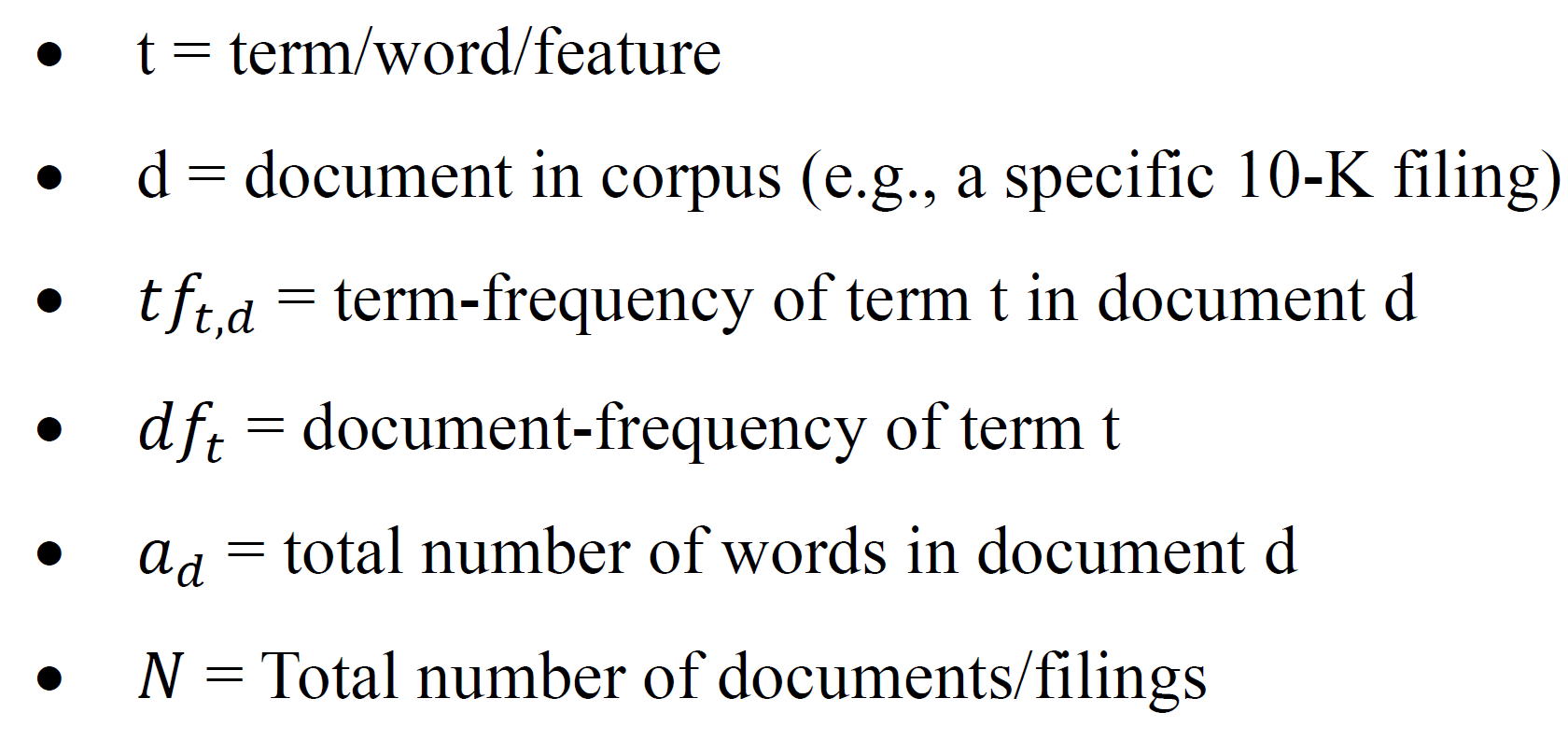
TF-IDF stands for “term frequency, inverse document frequency”. The basic idea behind TF-IDF is the fact that the more a word appears in a given document, i.e., the higher the term-frequency, the more representative that word is for that document. Hence, the weight of a word should increase with term-frequency. On the flip side, the opposite is true for document-frequency, which describes the number of documents that contain said word. The rationale for this lies in the fact that a word which is very common, i.e., that appears in most documents, does not contribute much informative value. Based on this weighting scheme, each word receives a different weight, and these weights will also differ across documents.
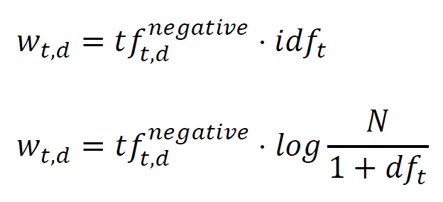
The weights for each word/term (t) within each document (d) are calculated as follows:
This is the standard implementation of TF-IDF as used by library scikit-learn. Internally, scikit-learn then also normalizes these weights. Consequently, this can be implemented with just a few lines of code:
In order to calculate the final sentiment score, the project follows the methodology proposed by Jegadeesh and Wu (2013). They propose to sum up the weights of all negative words per document and scale it by log of the total number of words per document. Accordingly, the normalized weights are used to obtain the final score as follows:
Data Collection and Organization
The data is organized in three tables. One table for the filings. A second table that contains the financial data as well as a third table corresponding to the used dictionary.
The textual data of the filings was downloaded using the official SEC-API. Company identifiers and other metadata was obtained by accessing the CRSP database through the W/R/D/S API. The entire download and filtering process is quite lenghty. For details I can kindly refer to the corresponding Jupyter Notebook with the commented code.
The filings-table (after filtering) contains 7,109 filings spread over 20 years with companies sorted into 20 different sectors according to the official NAICS labeling scheme.
Preprocessing Filings
Before the sentiment scores can be calculated the text of the filings are first being preprocessed. This step is crucial and, hence, takes up a large portion of the effort of the sentiment analysis. The entire process is visualized below:
Most of these steps are described by Gentzkow et al. (2019) who provide an overview of the process for integrating text into economic research. Consequently, all these steps are considered standard in various NLP tasks.
Reasons for preprocessing (see: Gentzkow et al., 2019, p. 536):
Standardize text
Ensuring appropriate data quality
Reduce dimensionality of the data rendering the subsequent process more efficient.
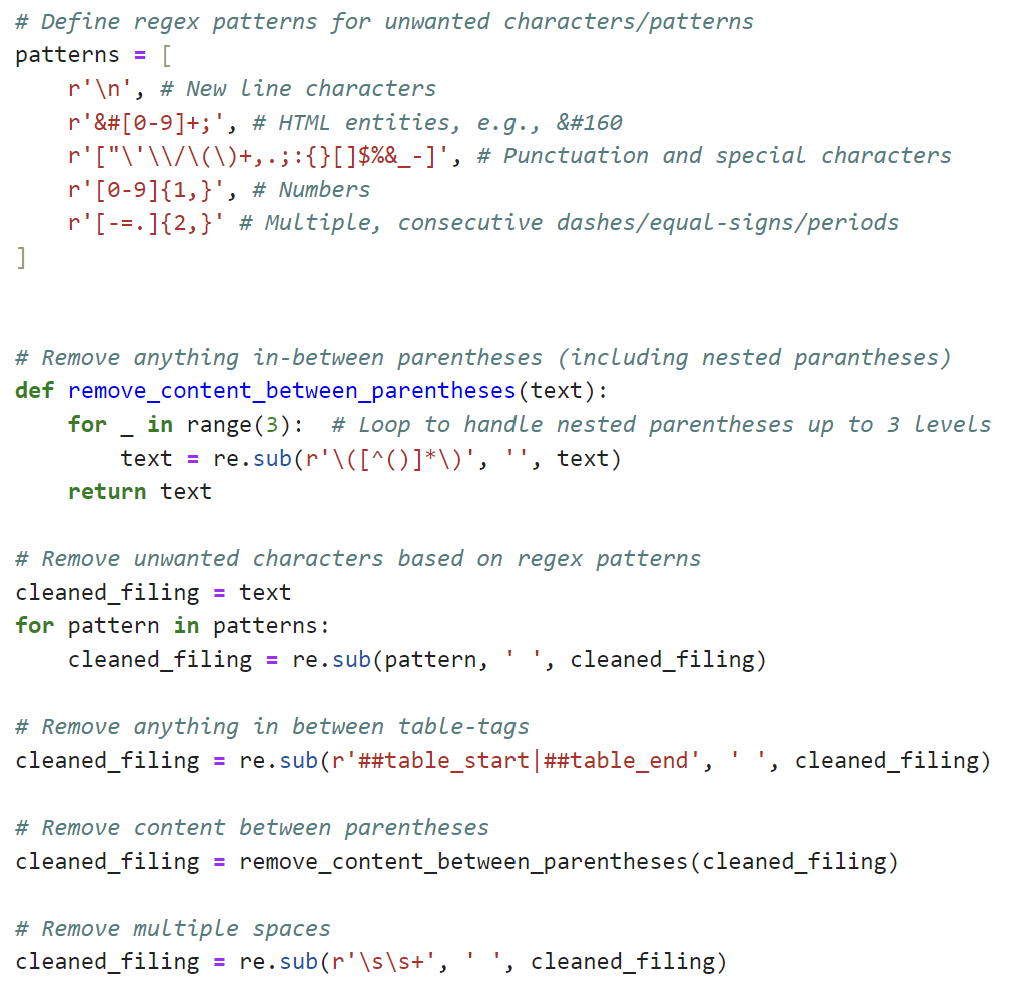
When removing unwanted characters it is common to remove punctuation, special characters, remaining HTML-entities, but also tables and especially numbers within them. The main idea behind removing numbers lies in the goal of sentiment analysis. Sentiment analysis aims to extract the sentiment conveyed by the text itself. Hence, the process is meant to capture information contained in the text that goes beyond purely quantitative information represented in numbers. Therefore, to be able to extract narrative rather than quantitative information, all numbers are removed.
This removal is handled through the use of regular expression (regex) with the help of the Python module “re”. Below the main central part of the corresponding custom Python is displayed.
The following step of tokenization is described by Manning and Schütze (1999, p. 124) as the process of splitting text into its preferred units, commonly referred to as tokens. The most common type of token is an individual word (unigram). In the code this handled by the word tokenizer and the corresponding function (word_tokenize(text)) of the NLTK library.
Additionally, it is desirable to treat different inflections or versions of a word as the same basic word. Generally, there are two prevalent approaches of doing that: Stemming and lemmatization. According to Manning et al. (2009, p. 46) the performance gain for either approach is not always clear. Given that both approaches aim to accomplish the same task, the final choice between stemming and lemmatization might be more of a personal decision. The analysis at hand uses lemmatization. Although lemmatization is computationally more expensive, it is also more sophisticated and less aggressive.
“Lemmatization is a process that maps the various forms of a word (such as appeared, appears) to the canonical or citation form of the word, also know as the lexeme or lemma (e.g., appear).” - (Bird/Klein, 2009, p. 121.)
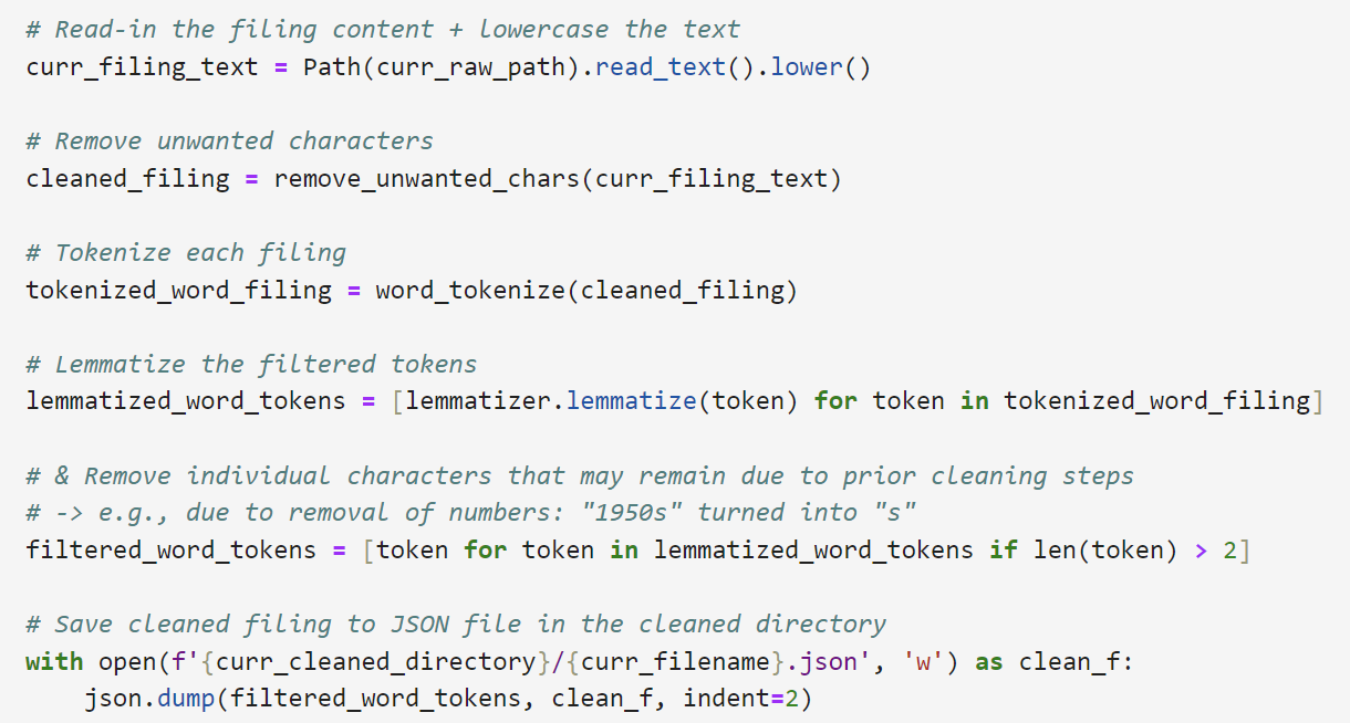
The final filtering step removes all tokens with less than three characters. Once again, this helps reduce noise as some of the prior cleaning and processing steps may have left behind some remaining pieces of tokens. For instance, removing numbers also means reducing the token ‘1960s’ to simply ‘s’. As single- or double-character words are hardly able to convey any meaning on their own, they are removed.
The code below showcases all aforementioned preprocessing steps that are performed within a for-loop on all available filings.
Exploratory Analysis
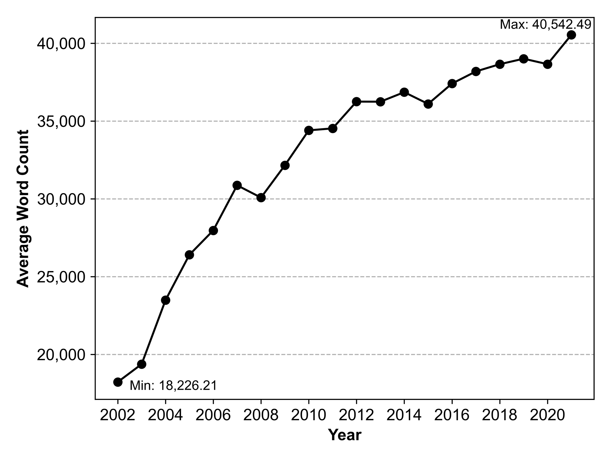
As initially mentioned, the focus now turns to identifying trends and patterns in the prepared dataset. First, I take a look at the filings themselves. The figure below shows the development of the average length per filing over the entire sample period. The average word count for 10-K filings increases almost monotonically. The surge is dramatic in size over the entire sample period as the average length more than doubles from 2002 to 2021.
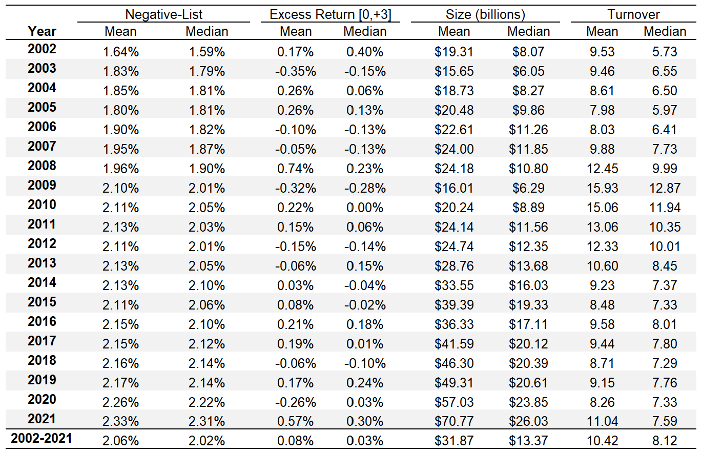
To get a feel for the data and sample at hand the next figure below displays some summary statistics and their development over the sample period.
The variable Negative-List shows the average percentage of negative words per filing. These percentages increase steadily over the sample period. Thereby, the analysis at hand can report a continuation of the upward trend that Loughran and McDonald (2011) report for their sample period ranging from 1994 to 2008. Naturally, the average market cap (size) of companies is noticeably larger in the project compared to Loughran and McDonald (2011). This is due to the fact that this analysis is limited to S&P 500 companies while the original study considers a much larger range of companies including smaller ones. Additionally, the sample period for these two studies ended a lot earlier (2008), whereas the present analysis stops in 2021. Between 2008 and 2021 S&P 500 companies experienced a notable increase in market cap.
The excess return, here, is calculated for the period [0, +3] using the BHAR (Buy-and-Hold Abnormal return) approach with the S&P 500 market return being the benchmark. No clear trend is visible here.
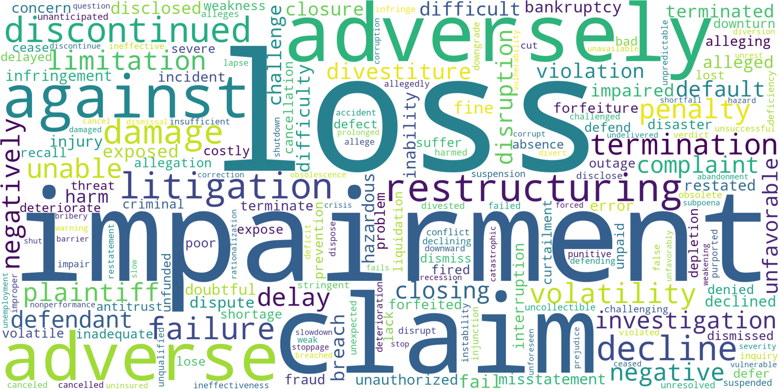
Before exploring the sentiment scores, the analysis first digs into what influences these scores—specifically, the negative words sourced from the dictionary. The word cloud below displays the most commonly used negative terms, with the size of each term indicating how frequently it appears. Clearly, words such as “loss”, “impairment”, and “claim” are the most common and, hence, will also have the largest impact on the sentiment scores.
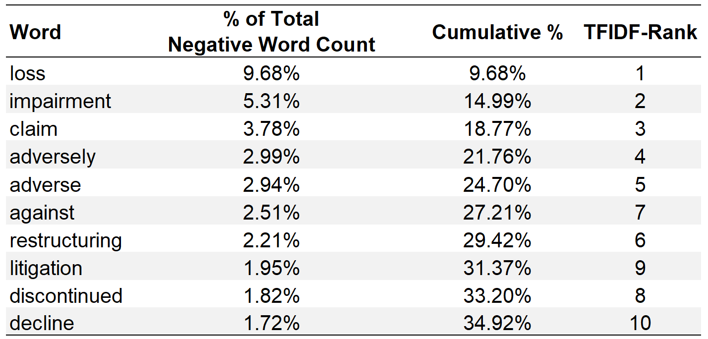
These observations can also be quantified by examining the most frequent words, as shown in the table below. Surprisingly, the top ten most common words account for more than one third of all negative word counts. This finding is unexpected considering the analysis encompasses nearly 2,000 distinct negative words. Interestingly, the corresponding TF-IDF ranks of these ten words indicate that the most common words are also deemed important when applying the TF-IDF scheme. In fact, the top ten words in terms of absolute frequency correspond percisely align with the top ten words according to TF-IDF, albeit with a slight variation in their order.
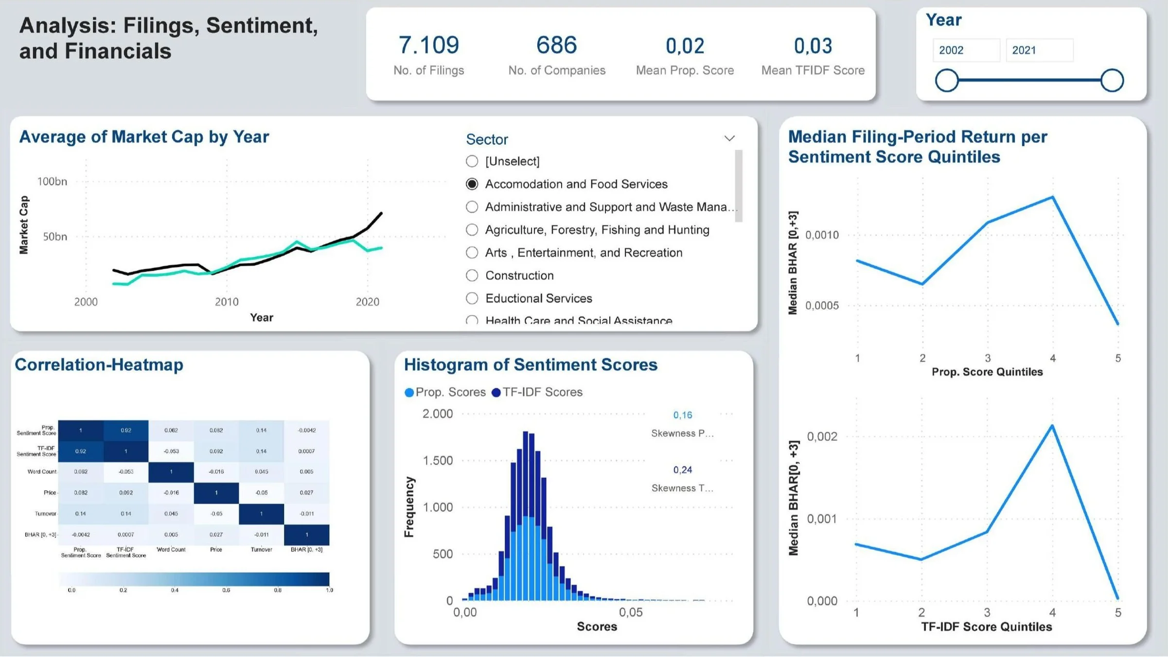
Given that the proportional sentiment scores rely on these relative frequencies, the significant overlap in the top ten suggests a notable interdependence between the proportional sentiment scores and TF-IDF sentiment scores. Across the entire sample, the proportional sentiment scores exhibit an exceptionally high correlation with the TF-IDF sentiment scores of approximately 0.92.
The Power BI dashboard below gives more insights into the data.

